Target Generation and Detection

Next, you will be simulating the signal propagation and moving target scenario.

Theory :

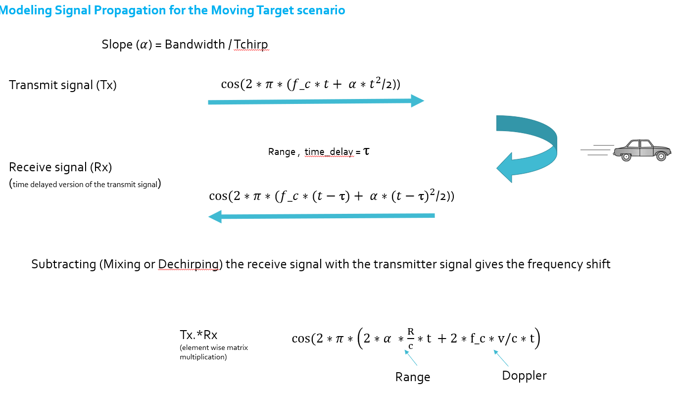
In terms of wave equation, FMCW transmit and received signals are defined using these wave equations, where α = Slope \,\, of \,\, the \,\, signal . The Transmit Signal is given by:

Tx= \cos(2\pi(f_ct + \frac{\alpha t^2}{2}))

The received signal is nothing but the time delayed version of the Transmit Signal. In digital signal processing the time delayed version is defined by (t -\tau) , where \tau represents the delay time, which in radar processing is the trip time for the signal.

Replacing t with (t -\tau) gives the Receive Signal:

Rx = \cos(2\pi(f_c(t-\tau) + \frac{α(t-\tau)^2}{2}))

On mixing these two signals, we get the beat signal, which holds the values for both range as well as doppler. By implementing the 2D FFT on this beat signal, we can extract both Range and Doppler information

The beat signal can be calculated by multiplying the Transmit signal with Receive signal. This process in turn works as frequency subtraction. It is implemented by element by element multiplication of transmit and receive signal matrices.

Mixed or Beat Signal = (Tx.*Rx)

The above operation gives:

Tx.*Rx = \cos(2\pi(\frac{2\alpha R}{c}t + \frac{2f_cvn}{c}t))